Fun Stuff - How to make a movie

Fun Stuff - How to make movies from sliding window data!

samslide.py

samslide.py is a Python script that lets you create SAM movies, either on a standalone machine or on the NIH Biowulf Cluster.

This script slides SAM time windows across a given interval using a given time-step, creating a series of consecutive SAM volumes which are saved as an AFNI 3d+time dataset. It can slide either or both of the active or control windows in a variety of ways.

The script's output is a set of shell scripts which are suitable for use on a standalone machine, but which were created for ease of use on the Biowulf cluster with the swarm command (hint: use the bundle mode (-b, see swarm -h) and use -l nodes=1:p2800 or similar). See also the Biowulf hints page.

Download and Installation

Download samslide.py. Make it executable and put it somewhere, perhaps somewhere along your $PATH.

Sliding Window SAM

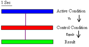
For an example of how samslide.py works, let's first look at a typical non-sliding SAM window used to calculate the difference between 5 seconds of active and control condition:

Typical SAM Analysis

This typical SAM usage results in a single .svl file (SAM's output) to show the differences from the active and control period over 5 seconds of data. This collapses the entire 5 second trial into a single difference.

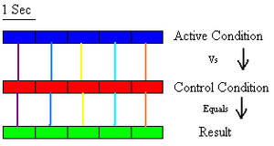
Now, if you are interested in what's going on at a finer time scale, for example you'd like to see signal differences second by second, your first instinct may be to use a "One to One" approach:

One to One approach

Here, each 1 second window in each condition is directly contrasted to its counterpart. This results in 5 .svl files, each representing the difference between 1 second of active and 1 second of control condition. If you do choose to take this approach, remember that each result window reflects the difference in the signals between the active and control states, so the actual result could be, and often is, driven just as much by variations in the control condition as the variations in the active condition.

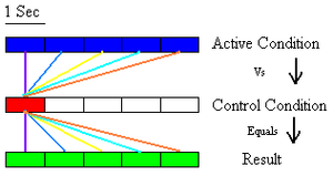
If you are more interested in variations in signals throughout your active condition than your control condition, you may choose to use samslide.py in a "One to Single" approach:

One to Single approach

Where each 1 second of active condition is contrasted against the same 1 second of control condition. In this approach, while each of the five result periods is driven just as much by the control condition as the active condition, the differences between each result file (as you look at each of the 5 results in sequence) is driven purely by the differences in the active condition. This can be very useful if you are looking for increases or decreases in certain signals over the active condition, as you can be certain that, if in your active condition the power in time segment one (second 0–1) for a given spatial location and frequency band is lower than that for time segment two (second 1–2), then between time period one and two that frequency band increases in power. While this approach is normally preferred compared to the previous, there are still some issues to keep in mind. For instance, if you are more interested in the difference between the active and control conditions than the differences throughout the active condition, then if your small control window is non-ideal (e.g., the subject was not 'resting' or doing the appropriate control task), all of your results will be very skewed.

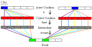
To compensate, you may want to use samslide.py in a "One to All Control" approach:

One to All Control approach

Here, only active time period 1 and 3 are illustrated to keep the example from becoming too bulky and confusing.

This approach contrasts each window in the active condition (or as illustrated, active window 1 and 3), with each window in the control period, then averages across the resulting movies to form the result windows. While this is by far the most computationally intensive method, it affords much more stability than all previous approaches when looking at the active condition. By comparing each active window with every control window, variation throughout the control condition has much less impact on the result. In addition, because no single control window is relied upon completely for contrast, a single window in the control period being non-ideal should not completely spoil your results.

General things to keep in mind about samslide.py

1. None of these methods should be approached as 'plug and chug.' MEG data is complex, and using multiple methods is highly recommended to see what is actually happening in your data. For instance, if you use the One to All Control method, you may see interesting results, however if you explore no further you might not find that throughout your control condition, instead of normal variation there is a trend that slants all of your results, so using a One to Single analysis could have shown even more insightful and interesting findings. In this case you might want to use several One to Single analyses, choosing several different control windows; or, a trend in your control condition could be detected by reversing the active and control conditions, and running a One to Single analysis sliding across your control windows. Ideally you should always think carefully about how you want to approach your data.

1. The number of trials is very important for samslide.py. For instance, in your experiment, you have 10 trials of active and control, each lasting 5 seconds. In typical SAM analysis you would have 50 seconds of active and control periods to contrast (10 Trials X 5 Seconds). This could be an acceptable amount of time to contrast, however if you used windows of 1 second, each contrast would only have 10 seconds of active and 10 seconds of control (10 Trials X 1 Second), which may not be adequate, causing inaccurate results. If you have questions concerning acceptable times for each condition it is advised that you contact MEG Core staff during your experimental design.

1. If you are interested in a smaller amount of time than regular SAM can accurately offer, you may want to use SAMerf. Also, you could overlap windows while keeping them large, for example you could use samslide.py to produce ~50 1 second windows for a 5 second time period, having each window start 0.1 second after the previous. However you should keep in mind that this is very different from a '0.1 second temporal resolution,' as each window is computed using an entire second from each trial in each condition.

The 5.0 CTF software is available on Biowulf under /usr/local/ctf/bin. Add that to your PATH, and set CTF_DIR to /usr/local/ctf. You probably want to add /usr/local/afni/linux_gcc32 to your PATH as well. The Biowulf login node can't run this version of AFNI, but if you request an interactive node (qsub -I -l nodes=1), you can run the assemble scripts using the gcc32 version of AFNI on the interactive node.

Usage: samslide.py [options] -g dataset.ds

This will create all the scripts and run them.

On the Biowulf one might do:

samslide.py [options] dataset.ds > batch samslide.py [options] dataset2.ds >> batch ... swarm -f batch -b [bundle size] -l nodes=1

Running the script with no arguments produces a detailed help message.

samslide.py outputs a script (here, batch) that you can append to in subsequent invocations with '>>'. The idea is that you want to do as many SAM runs as possible in one batch, to reduce overhead and waiting time.

The bundle size should be the number of lines in batch divided by the number of processors you expect to get. There are two processors per node. Thus, if you have 800 lines in batch, and you use 50 nodes (100 processors), specify -b8.

Note: samslide.py modifies the datasets! It creates window parameter files in the $ds/SAM subdirectory; it also creates go, assemble, and cleanup scripts in the current directory; a copy of the output, a script to assemble the final output BRIK, and one to clean up the various temporary files, respectively. If you are running many subjects/datasets at once, be careful to set the -t flag argument so that you avoid name collisions.

Viewing the Results in AFNI

Here's how to set up AFNI to view a movie:

1. Run afni. happy smiley
2. Set the Underlay to the anatomy.
3. Open some Image windows.
4. Set the Overlay to the movie (3d+t dataset).
5. Click "See Overlay".
6. Hit "New" (opens a new controller window).
7. In the new controller [B], set the Underlay to the same movie.
8. Also in the new controller, open a Graph.
9. Then, in Define Datamode, Lock, and Time Lock.

Now you can set your colors and graph preferences, and navigate in both time and space. It's a good idea to turn autoRange off, and set it manually.

For graph preferences, try setting the matrix size to 5 or 7, set a common or global baseline ('b' key), and autoscale ('a' key). The 'w' key writes the graph in the middle.